 This post describes a simple, robust, and repeatable workflow for processing astronomical images in Siril from an OSC (one-shot color) camera.
It is not an advanced or optimized workflow. It is a workflow designed for:
- those who are just starting out
- those who want consistent results
- those who want to learn how to control noise, rather than trying to correct it at the end
This workflow assumes that Siril is already correctly installed and configured. If you haven't done so yet, start with the previous post on installing and configuring Siril.
By following the steps in order and taking your time, you can obtain balanced images with a controlled background and credible colors.
1 — Prepare the working folder
Create a main work folder and, inside it, the following subfolders:
- lights
- darks
- flats
- biases
If the files already exist on another disk or in another location, use symlinks instead of copying the data. You avoid duplication, save space, and keep everything organized.
A clean structure prevents errors and facilitates all processing.
2 — Choose the working folder in Siril
Open Siril and select the main working folder you created:
3 — Preprocessing and stacking (automatic)
Run the preprocessing script:
- Scripts → Siril script files → OSC_Preprocessing
This step automatically handles:
- calibration (darks, flats, and bias)
- image alignment
- final stacking
If you do not have all calibration frames
Choose the most appropriate script:
- OSC_Preprocessing_WithoutDark
- OSC_Preprocessing_WithoutFlat
- OSC_Preprocessing _WithoutDBF
Important note: less calibration means more noise. This is not a limitation of Siril, it is a physical consequence of the data.
4 — Open the resulting image
Open the file created by the script - Open → result_xxxx.fit
The "xxxx" is the total number of seconds of exposure.
The image will appear dark, lacking contrast, and uninteresting. This is normal. At this point, the image is still linear.
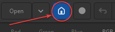
5 — Display mode: Stretch (visualization)
|
|
Change the display mode to AutoStretch (1). If the image has very strong color casts, use Unlink channels (2). This stretch is only visual. It does not change the image data.
|

6 — Crop
Draw a rectangle over the image to exclude irregular edges or areas with incomplete stacking. Anything outside this area only adds noise and makes the following steps more difficult.
You can drag the sides to adjust or click outside the rectangle to start over.
Right-click to bring up the rectangle – Crop – Crop.
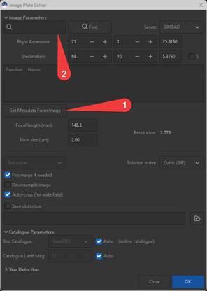
7 — Plate solving (astrometry)
|
|
Run the plate solver:
Use the "Get metadata from image" button (1). If the data is filled in, just click "OK." If not, search for the DSO in question (2).
This step is essential for modern color calibration (SPCC).
If it fails, solve the problem now; do not proceed without this working. |
8 — Background Extraction


Use few, well-placed samples. A poorly done BGE creates more problems than it solves.
9 — Color calibration (SPCC)
Calibrate the image color:
- Image Processing → Color Calibration → SPCC
- Choose the sensor and filter used
If plate solving was successful, this step is straightforward.
Completely unrealistic colors indicate problems in previous steps
10 — Return to linear
Change the display mode again:
- Display Mode → Linear
From here on, all changes will modify the image data.
11 — Stretching (where noise becomes visible)
Noise does not appear in this step — it was already present in the data. Stretching simply makes it visible.
Fundamental rule

The more aggressive the stretch, the more noise you will see.
Image Processing – Stretches – Curves Transformation
- By clicking on the diagonal line, you add control points. Create one point near the bottom and another near the center. Pull the bottom point slightly down and the top point slightly up. Observe the result. Apply smooth adjustments to the curve, in an S shape.
- Avoid excessive slopes
It is preferable to take several small steps rather than a single aggressive stretch.
13 — Final touches
Make only minor adjustments:
- If the image has a green tint, select Image Processing – Remove Green Noise and click Apply
- contrast
- moderate saturation
- subtle color corrections
If you feel the need for heavy corrections, the problem lies in previous steps of the workflow.
14 — Save the image
Save the final result:
- TIFF for external editing (Photoshop, GIMP, etc.)
- JPEG for publication
Always save an intermediate version. You will want to go back later.
Key idea for beginners
A good image is not the most stretched one.
It's the one that maintains a clean signal, controlled background, and credible colors, even if that means leaving some weak details unshown.
When you feel like you're fighting noise, you're probably asking more of the image than the data actually allows.